Tutorial Corner - Giant Steps Part I - Basics and Pitch
Giant Steps
The aim of this tutorial is to introduce some main functions of the MeloSpyGUI. Additionally, you will see how the MeloSpyGUI and the Weimar Jazz Database can be used when working on certain research tasks. Using John Coltrane’s “Giant Steps” (1959) as an example, several features for comparing melodic, intervallic, and rhythmic details will be explained. Furthermore, Coltrane’s usage of tonal patterns is to be explored, using the pattern search engine of the MeloSpyGUI.
As Coltrane played two solos in the same recording of “Giant Steps”, you may compare improvisational strategies of one soloist in the same piece - this can be of interest if creativity and redundancy in jazz improvisations are to be explored. Since “Giant Steps” was frequently discussed in jazz studies and music psychology over the last decades (e.g. Ake 2010: 20-24; Behne 1990; Jost 1980; Lehmann/Goldhahn 2016), one main aim of this tutorial is to show how computer aided analysis of jazz soli might complement rather established methods such as transcriptions. Lehmann and Goldhahn (2016: 352), for example, highlight the challenge of improvising to “Giant Steps” since the chord structures are quite complex and the tempo is pretty high. It could be argue that playing and combining several memorized patterns might be one strategy to deal with such challenges. Additionally, Jost (1980) has already demonstrated Coltrane’s usage of very long patterns in “Giant Steps”. Using the analysis features of the MeloSpyGUI, previous research can be complemented by systematically describing such musical features in jazz improvisations.
The Data Tab
Let’s start the MeloSpyGUI. First of all, you have to select your data (Fig. 1). You can choose between two databases - Weimar Jazz Database (wjazzd.db) and Essen Folksong Database (esac.db) - or use your own external files. Choose wjazzd.db, and on the right you see a list of all solos currently contained in the Weimar Jazz Database.
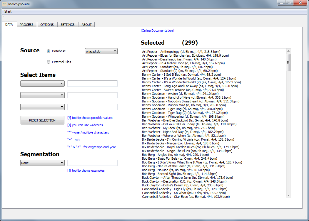
Fig. 1. MeloSpyGui Data Tab.
Now you can select your items: the performer (John Coltrane) and the title (Giant Steps) by using the drop down menus (Fig. 2). There are several further options, e.g. choosing certain kinds of rhythmic feel or tonality. Additionally, you can choose single segments of one or several solos such as bars, choruses, or phrases.
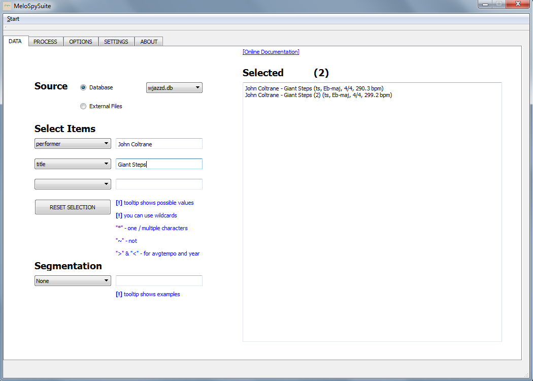
Fig. 2. Selection of Giant Steps.
Note: You can get further information about the several options by positioning the cursor on the field next to your selected item or segmentation (Fig. 3). After choosing the data, you can go on to the Process tab.
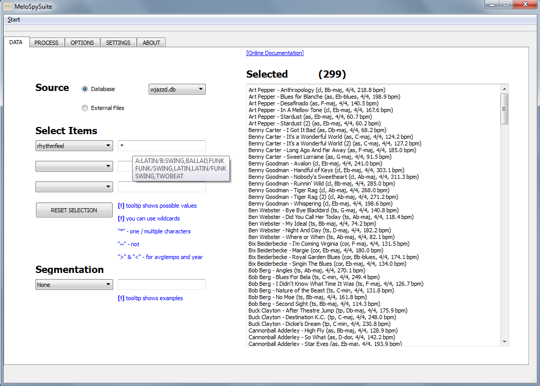
Fig. 3. MeloSpyGui tool tips.
The Process Tab
The process tab contains three different modules: feature + visualization, pattern, and convert - at first, have a look at feature + visualization. This module allows you to choose between 14 main feature categories - in alphabetical order from accents to tone formation - and countless subcategories for detailed analysis. At the beginning, you may collect some basic information about the recording by choosing the category metadata and the subcategory general_solo_metadata. For example, you want to inform yourself about the recording year, basic musical features such as tempo, key, and tonality, the played instruments, and the number of choruses of Coltrane’s solos. So you choose recordingyear, avgtempo, key, tonality_type, instrument, and chorus_count. In this case, you don’t need any visualization, so you choose no (feature extraction only) in the visualization drop down menu.
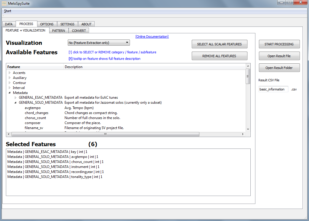
Fig. 4. Selecting metadata as features.
The chosen information will be listed in a csv-file which you can name, for example, basic_information (Fig. 4). Note: It might be necessary to change the options for Decimal point, depending on the version of Excel or Calc you are working with; you can change the options when switching to the OPTIONS tab. Then click start processing and afterwards open result file (Fig. 5).
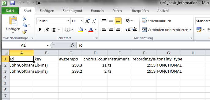
Fig. 5. CSV file with metadata.
For a quite basic visualization of the melodic contour of the two solos, you can choose piano roll in the visualization drop down menu. The piano roll view provides a rough overview of the pitches and the duration of each solo (Fig. 6 and 7). One sees that Coltrane’s first solo is much longer (1127 notes) as the second (198 notes).
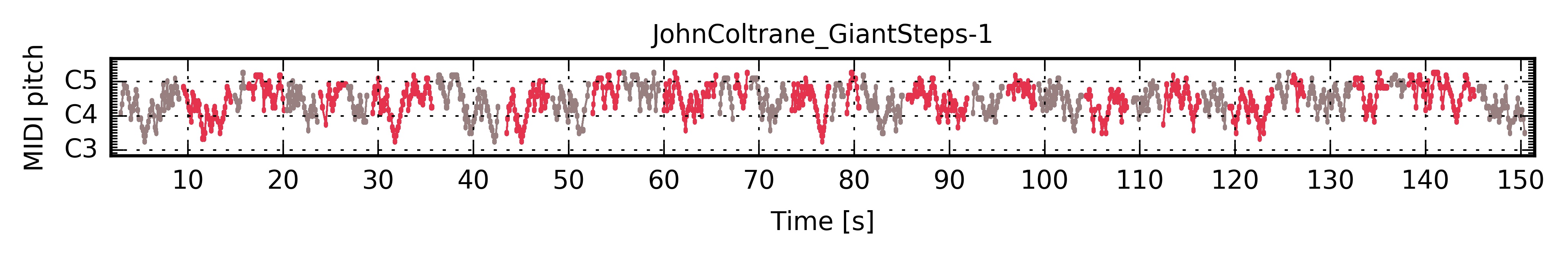
Fig. 6. Piano roll representation of Coltrane’s first solo on Giant Steps.
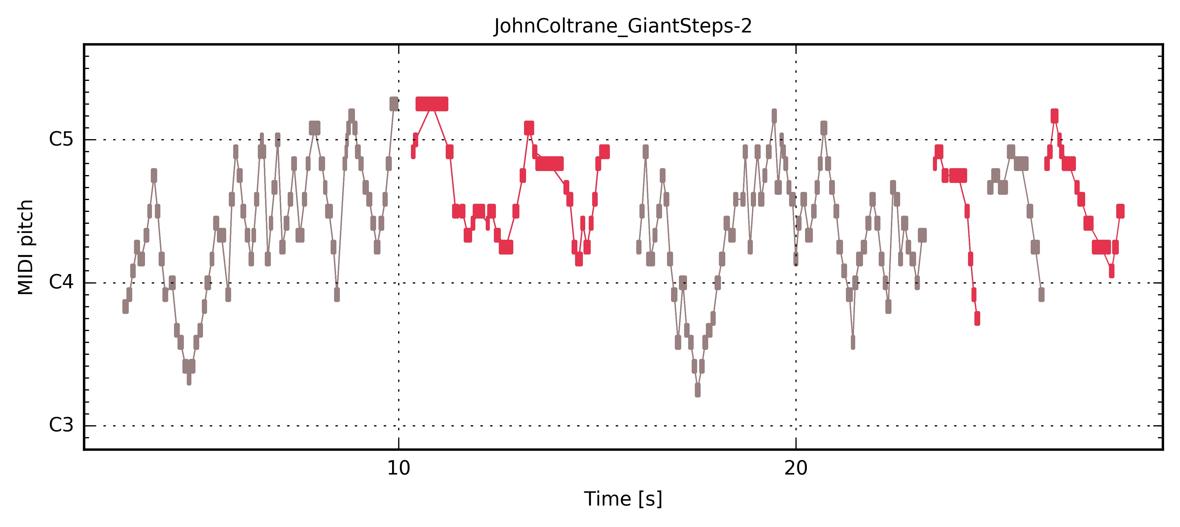
Fig. 7. Piano roll representation of Coltrane’s second solo on Giant Steps.
After collecting rather basic information, you can go on working on concrete research tasks. When listening to Coltrane’s improvisations on “Giant Steps”, it seems quite obvious that there are several similar tonal patterns in both solos. Moreover, the aforementioned results of previous publications confirm this impression. In order to get more detailed information about Coltrane’s tonal choices on the one hand and about similarities between the two solos on the other hand, you can use the MeloSpyGUI-features for pitch analysis.
Pitch
The pitch features allow you to analyze the pitches played by a soloist and to visualize the results with histograms. There are two general options for the visualization: Firstly, bar plot (over items) which means that one histogram will be created for each of the chosen features. Secondly, bar plot (over features). When choosing this option, you will get all chosen features listed in one histogram for each solo. For the comparison of Coltrane’s two solos on “Giant Steps”, you choose bar plot (over features) - so an overview of all pitches played in each solo will be given. First of all, you have to choose Pitch in the list of available features. Let’s say that you simply want to know which pitches are played most often in the solos. In this case you choose PC_FEATURES - PC stands for pitch classes. Then you can decide which features you will need for your analysis. To get an overview, it will be sufficient to choose the twelve pitch classes from C to B. Just right click on “pc_hist_density_00_C” and so on, and the features will be listed under “Selected Features” (Fig. 8).
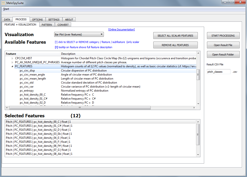
Fig. 8. Selection of pitch class features.
Then click start processing and have a look at the histograms which will be saved in the results folder (Fig. 9 and 10). As you can see, there are already some similarities. For example, Coltrane is barely playing C# and A while G, D, Eb, and B - especially in the second solo - are occurring quite often. Since you know the tonal center of the piece - Eb-major, see the metadata csv-file - you can already start to interpret Coltrane’s pitch choices.
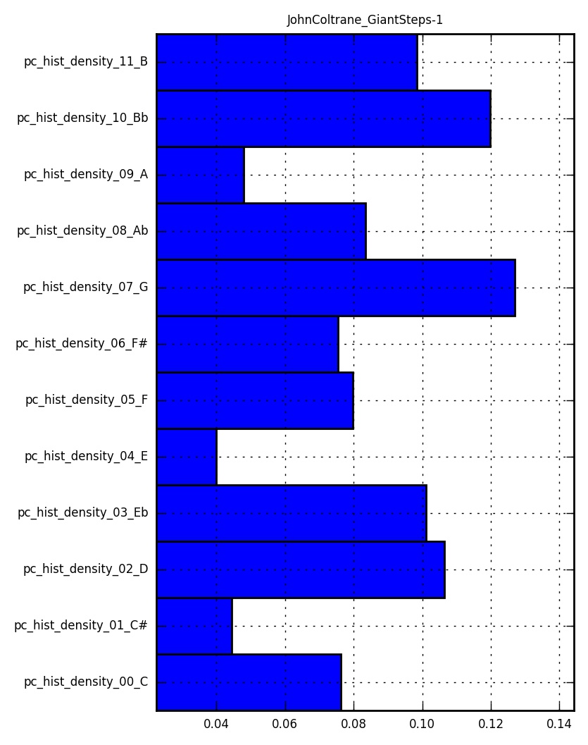
Fig. 9. Distribution of pitch classes in Coltrane’s first solo on Giant Steps.
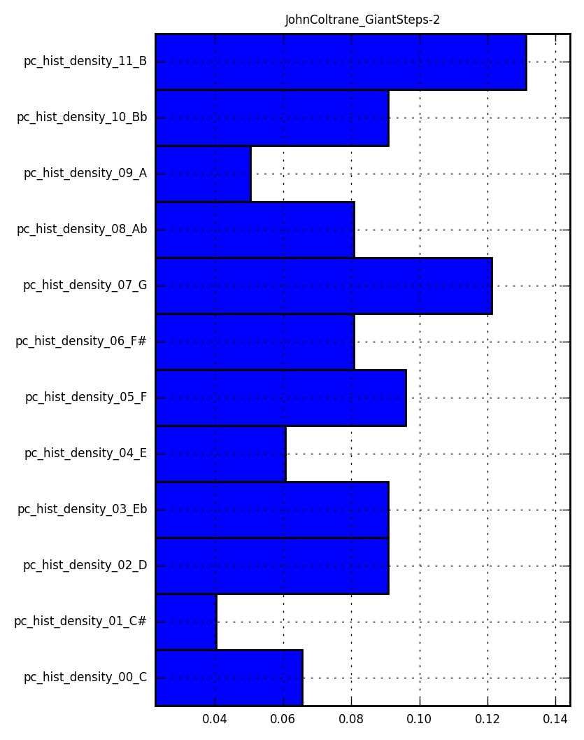
Fig. 10. Distribution of pitch classes in Coltrane’s second solo on Giant Steps.
But you can go deeper into detail. For instance, it could be of interest which pitches Coltrane has played in reference to the underlying chords. In this case you can choose CPC_FEATURES - that is, chordal pitch classes (CPC, see Chordal Pitch Class) will be analyzed. Repeat the work steps explained in the paragraph before and have a look at the cpc-histograms - 00 stands for the chord roots (Fig. 11 and 12).
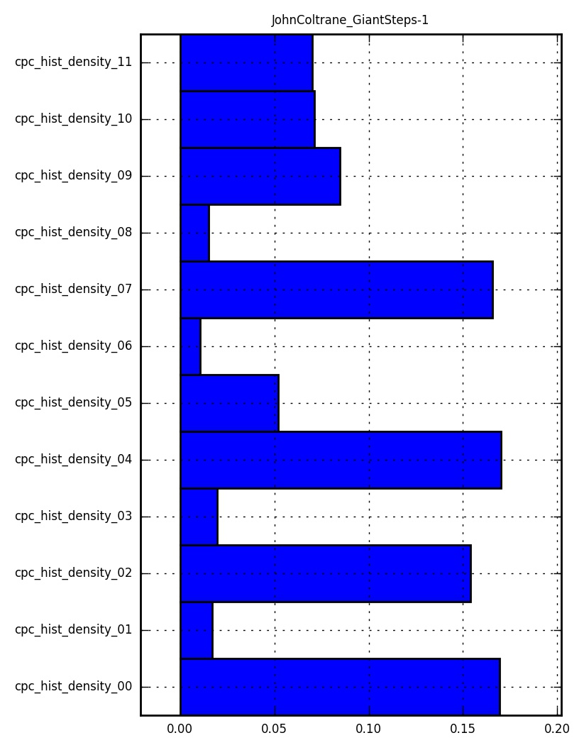
Fig. 11. Distribution of chordal pitch classes in Coltrane’s first solo on Giant Steps.
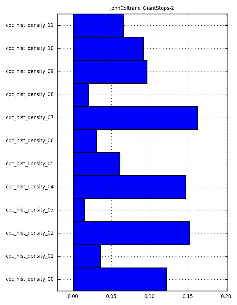
Fig. 12. Distribution of chordal pitch classes in Coltrane’s second solo on Giant Steps.
When comparing the two histograms, you can clearly see that there are only small differences. Coltrane emphasizes 00, 02, 04, and 07 while rather ignoring 01, 03, 06, and 08 - the difference is always less than five percent. So Coltrane clearly focuses on the root note, major second, major third, and fifth in reference to the accompanying chords in both solos. Now you have overview of the pitch classes in a chromatic order. But you can also generate histograms in a diatonic order. There are two different options: CDPC_FEATURES, and CDPCX_FEATURES; the latter provides more detailed information. Not only are the diatonic pitch classes from 1 to 7 listed, but also minor second (b2), minor sixth (b6), minor seventh over major (<), major third over major (>), tritone (T), minor third over major (B), and major seventh over minor (L) (see Chordal Diatonic Pitch Class and Extended Chordal Diatonic Pitch Class). Again, choose the features, click Processing and have a look at the histograms. Once more, the distribution of pitch classes looks quite similar and Coltrane’s emphasis on root note, second, third, and fifth becomes obvious. Note: you can save the settings for upcoming research or to continue working on certain examples to a later point in time: just switch to SETTINGS and label the current setting.
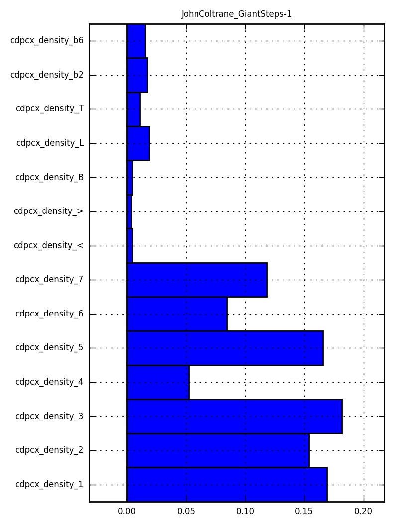
Fig. 13. Distribution of diatonic chordal pitch classes in Coltrane’s first solo on Giant Steps.
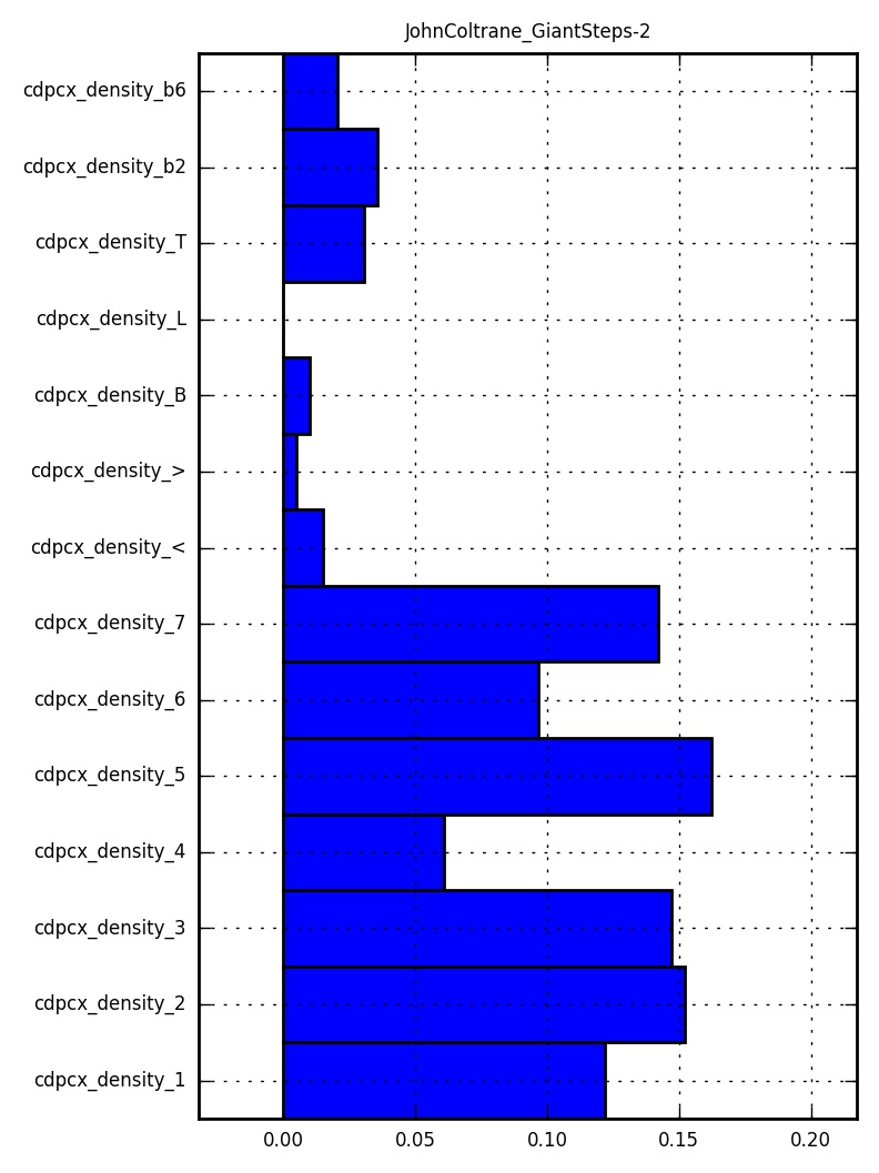
Fig. 14. Distribution of diatonic chordal pitch classes in Coltrane’s first solo on Giant Steps.
One further option for an analysis of pitch without generating histograms with the MeloSpyGUI is to count the melody notes played by a soloist. In doing so, select PITCH_HIST and then pitch_raw. The results will be displayed in a csv-file and can be used for further investigation with the software of your choice. For instance, you could explore the frequency distribution of the played notes. As you can see in Fig. 15 and 16, most of the absolute pitches played by Coltrane in both his two solos lie within the same range, between D4 and B4 (with G4 as the most frequent tone). However, there are some differences between the two frequency distributions which could be further explored in detail.
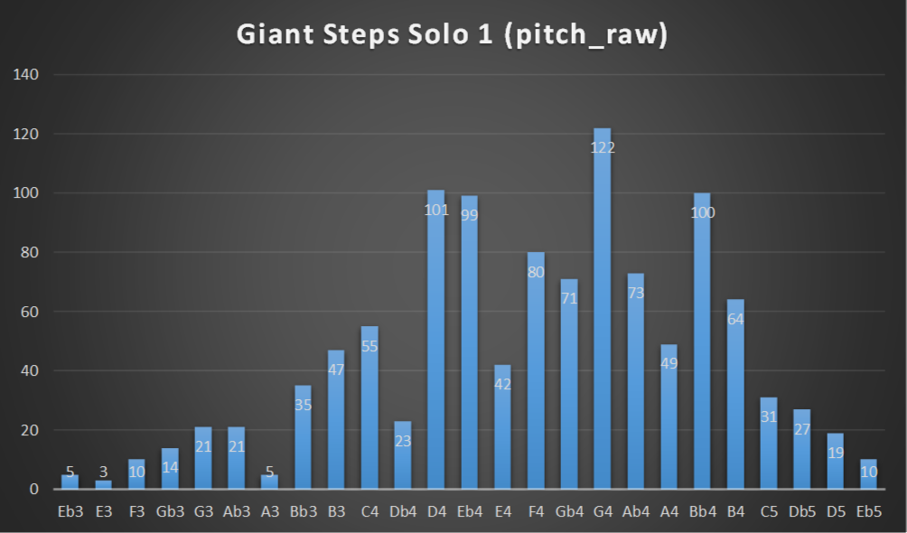
Fig. 15. Distribution of pitches in Coltrane’s first solo on Giant Steps.
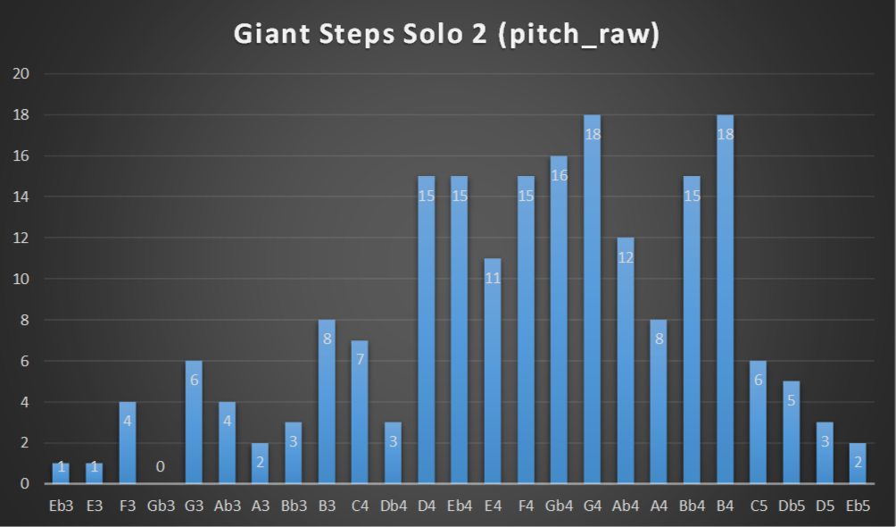
Fig. 16. Distribution of pitches in Coltrane’s second solo on Giant Steps.
To sum up: by using just a few of the available features for pitch analysis, you get detailed information about Coltrane’s pitch choices in a few seconds. It further enables you to compare the two solos of “Giant Steps”. Regarding pitch classes, the solos are distinctively similar. In a next step you may explore if the analysis of interval features will lead to comparable results. If your are interested in further possiblities for analyzing pitch, please check out our list of feature definition files.
© 2017References
Ake, David (2010). Jazz Matters. Sound, Place, and Time Since Bebop. Berkeley/Los Angeles: University of California Press.
Behne, Klaus-Ernst (1990). “Zur Psychologie der (freien) Improvisation”. In: Klaus-Ernst Behne, Gehört - Gedacht - Gesehen. Zehn Aufsätze zum visuellen, kreativen und theoretischen Umgang mit Musik. Regensburg: ConBrio, 113-130.
Goldhahn, Stephan and Andreas C. Lehmann (2016). “Duration of Playing Bursts and Redundancy of Melodic Jazz Improvisation in John Coltrane’s ‘Giant Steps’”. In: Musicae Scientiae 20(3), 345-360.
Jost, Ekkehard (1980). “Spontaneität und Klischee in der Jazzimprovisation, dargestellt an John Coltranes ‘Giant Steps’”. In: Hellmut Kühn and Peter Nitsche (Ed.), Bericht über den Internationalen Musikwissenschaftlichen Kongreß Berlin 1974. Bärenreiter: Kassel 1980, 457-460.
Next: Part II of the tutorial.